Results Gallery

Publication figures from the production dark-siren H₀ campaign run_20260620_seed500_phase50 — a single homogeneous catalogue of 1385 simulated EMRI detections evaluated on an 83-point super-dense H₀ grid (injected truth h = 0.73). All figures use the Observatory + Atlas design system (method→colour grammar, Planck/SH0ES reference bands, flat-prior overlay, nested HDI, Crameri scientific colormaps).

Combined-posterior MAP estimates:

• Without M_z (1D): h = 0.737 (+1.0 %)

• With M_z (2D): h = 0.732 (+0.3 %)

All figures are produced by the package itself via python -m master_thesis_code <simulations_dir> --generate_figures <simulations_dir> (the cluster PDFs are converted to PNG for web display).

H₀ inference

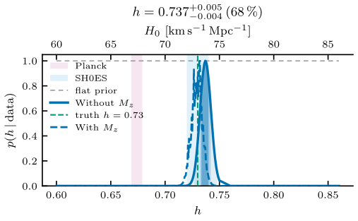
fig01 — Combined H₀ posterior. Catalogue-combined posterior for both mass conventions as one blue separated by linestyle (solid Without M_z, dashed With M_z), with nested 50/68/95 % HDI shading, the flat H₀ prior, Planck (pink) and SH0ES (cyan) bands, a km/s/Mpc top axis, and the MAP in the title.

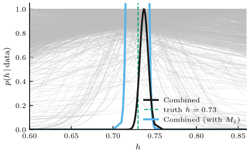
fig02 — Per-event posteriors. Peak-normalised single-event H₀ likelihoods coloured by SNR (batlow), with the catalogue-combined posterior as the black headline curve.

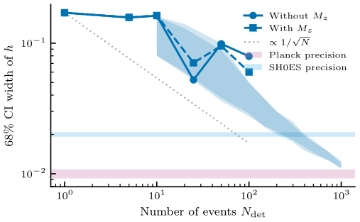
fig08 — H₀ convergence. 68 % credible-interval width as a function of the number of stacked detections, with the 1/√N guide and Planck/SH0ES target-width reference bands; mass conventions by linestyle.

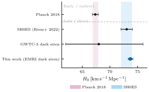
fig15 — H₀ in context. This work against Planck 2018, SH0ES (Riess+ 2022), and GWTC-3 dark sirens, sharing the same Planck-pink and SH0ES-cyan bands as fig01.

Detection catalogue & cosmology

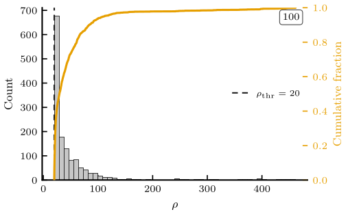
fig03 — SNR distribution. Signal-to-noise distribution of the detected catalogue (grey histogram) with the cumulative fraction and the detection threshold rule.

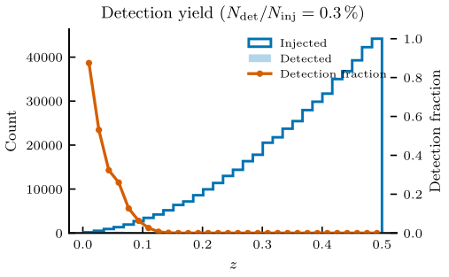
fig04 — Detection yield. Injected vs. detected redshift distribution from the injection campaign (504k injected; SNR ≥ 20 detected) with the per-bin detection fraction.

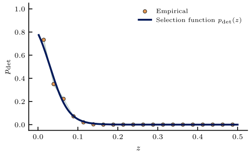
fig09 — Detection efficiency. Empirical detection probability vs. redshift from the injection pool with a smooth selection-function fit.

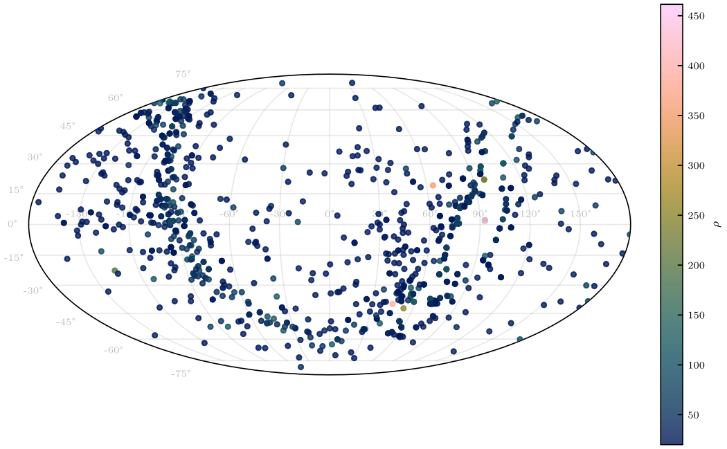
fig05 — Sky localization. Mollweide distribution of the detected events coloured by SNR (batlow).

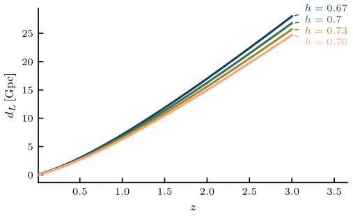
fig11 — Distance–redshift. Luminosity distance d_L(z) [Gpc] for a family of H₀ values, direct-labelled at the curve endpoints.

Parameter estimation

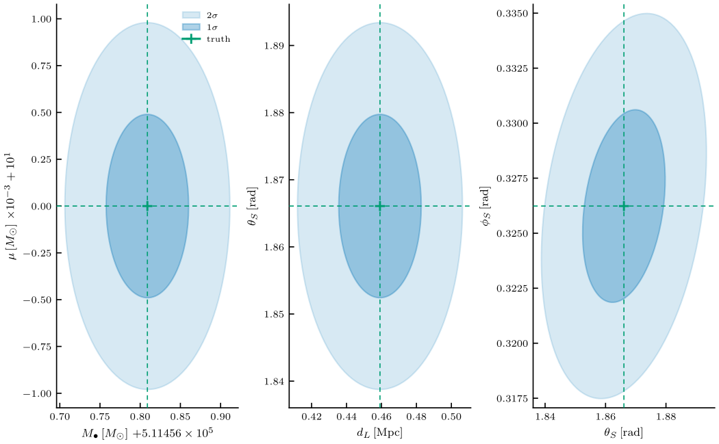
fig06 — Fisher ellipses. 1σ/2σ Fisher-matrix uncertainty ellipses for a representative event, with the truth crosshair.

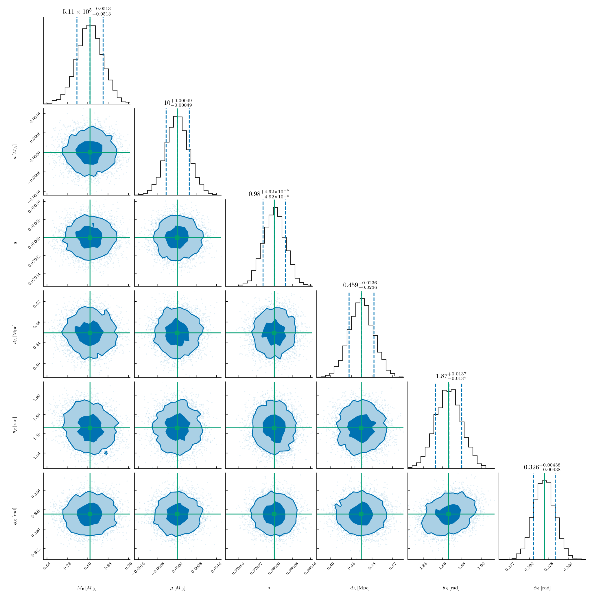
fig07 — Corner plot. Analytic Fisher parameter covariances (no KDE smoothing) at 1σ and 2σ.

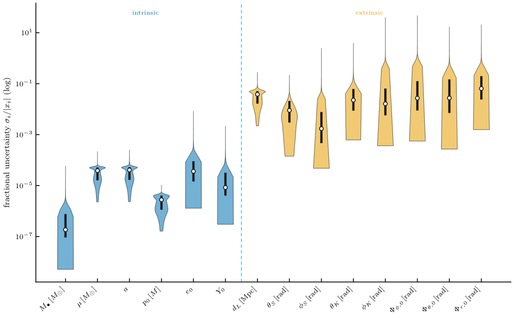
fig12 — Uncertainty violins. Per-parameter fractional Cramér–Rao uncertainties, split into intrinsic and extrinsic groups.

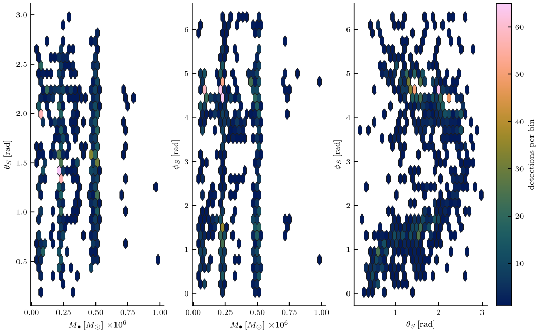
fig14 — CRB coverage. 2D pairwise hexbin density of the detected events across the key parameter pairs (batlow).

Instrument & signals

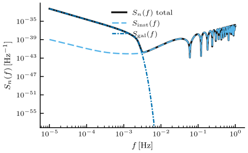
fig10 — LISA PSD. A-channel noise PSD decomposed into instrument and galactic-confusion contributions (distinguished by linestyle).

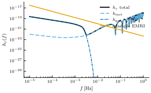
fig13 — Characteristic strain. Characteristic strain with a representative EMRI inspiral track against the LISA sensitivity.